Vortex-induced Vibration and Rotational Motion
Advised by Prof. Haecheon Choi and Dr. Daeun Seo at the Turbulence, Flow Control and CFD / Bio-Mimetic Engineering Laboratory (TFC), Seoul National University.
What’s Vortex-Induced Vibration?
When fluid flows past a bluff body — a cylinder, a bridge cable, an offshore riser — vortices shed alternately from each side, creating periodic forces that make the structure oscillate. This is vortex-induced vibration (VIV), and it’s one of the classic problems in fluid-structure interaction (FSI). At certain flow speeds, the vortex shedding frequency locks onto the structure’s natural frequency (a phenomenon called lock-in), causing large-amplitude oscillations that can be dangerous in engineering applications.
Most VIV research focuses on circular cylinders, but many real-world structures have elliptical or non-circular cross-sections. Elliptical cylinders behave differently — their aspect ratio changes how vortices form and how the structure responds. Prior work by Wang et al. (2019) studied elliptical cylinders with 2 degrees of freedom (transverse vibration + rotation), but the full 3-DOF case (adding streamwise vibration) hadn’t been explored.
The Goal
My thesis aimed to simulate the VIV and rotational motion of an elliptical cylinder with 3 degrees of freedom (x-translation, y-translation, and rotation θ) using the Weak Coupling Method, and compare the results against existing 1-DOF and 2-DOF studies.
The Weak Coupling Method
Solving FSI problems requires coupling the fluid equations (Navier-Stokes) with the structure’s equations of motion. The standard approach — strong coupling — iterates between the two until convergence at each timestep, which is expensive. The Weak Coupling Method (Kim et al., 2018) avoids this by using a predictor to estimate the structure’s provisional displacement and velocity, then solving the fluid and structure equations just once per timestep. It’s much cheaper computationally while still producing accurate results, especially for problems where the solid-to-fluid density ratio is low.
I implemented this in Fortran, using a discrete-forcing immersed boundary method for the fluid solver and the generalized-α method for time integration of the structural equations. The equations of motion for all three directions were non-dimensionalized and solved independently at each timestep using force coefficients (drag, lift, and moment) computed from the flow.
Setup
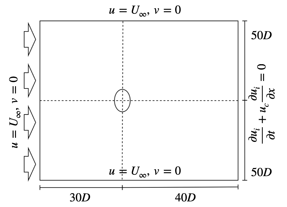
The elliptical cylinder had an aspect ratio (AR) of 2.0, and simulations were run at Reynolds number 150. The computational domain spanned 70D × 100D with roughly 820,000 grid points, refined near the cylinder where vortex dynamics matter most. I varied the reduced velocity U* from 3.0 to 13.0 to sweep through the lock-in region and beyond.
Results — Honestly Mixed
The validation worked well. Free and forced vibration tests of the structural solver matched analytical solutions exactly. The stationary cylinder simulation reproduced known values of drag coefficient, lift coefficient amplitude, and Strouhal number from the literature.
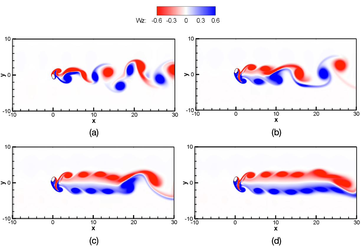
The 3-DOF VIV results were more nuanced. In the lock-in region, things looked good: all three directions (x, y, θ) vibrated at the same frequency, confirming that lock-in synchronizes all degrees of freedom — not just the ones studied in 2-DOF models. The vortex patterns showed clear 2S* mode shedding across all DOF configurations.
| DOF | X_max/D | Y_max/D | θ_max | f_x | f_y | f_θ |
|---|---|---|---|---|---|---|
| x only | — | 1.096 | — | — | 0.191 | — |
| x, y | 0.194 | 1.578 | — | 0.194 | 0.193 | — |
| y, θ | — | 1.085 | 0.493 | — | 0.195 | 0.195 |
| x, y, θ | 0.192 | 1.090 | 0.497 | 0.195 | 0.195 | 0.195 |
However, outside the lock-in region, discrepancies appeared compared to Wang et al.’s 2-DOF results. The frequencies diverged, and while amplitudes in x and θ stayed similar, the y-direction maximum displacement differed noticeably. This wasn’t entirely surprising — the Weak Coupling Method trades some accuracy for speed, and these differences grew at reduced velocities where lock-in breaks down.
The parametric sweep over reduced velocity showed that lock-in occurs roughly between U* = 4.0 and 7.0, with amplitudes growing dramatically in that range (Y_max/D reaching nearly 2.9 at U* = 7.0). Beyond U* = 8.0, the vibration amplitudes became too large to report meaningful steady-state values for some configurations, marked as dashes in the results table.
Overall, the study confirmed that the number of degrees of freedom affects when and how lock-in occurs, and that the 3-DOF model captures phase synchronization across all directions. But the quantitative agreement with prior work was limited outside the lock-in region, suggesting that the Weak Coupling Method’s approximations have a measurable impact in those regimes.
What I Learned
This was my undergraduate thesis and my first real experience with computational fluid dynamics beyond coursework. A few takeaways:
CFD is slow, and patience is a skill. Each simulation took hours to days on the lab’s cluster. I spent a lot of time waiting for results, debugging Fortran code, and re-running cases when parameters were off. The turnaround time forced me to think carefully before launching each run rather than iterating quickly.
Validation is not optional — it’s the foundation. Before running any VIV case, I had to verify the structural solver (free/forced vibration) and the fluid solver (stationary cylinder) independently. Without that, I’d have had no way to tell whether discrepancies in the coupled results came from the physics, the numerics, or a bug. This discipline has stuck with me in every project since.
Simplifications have consequences you can measure. The Weak Coupling Method is elegant and efficient, but the thesis showed concretely where it starts to lose accuracy. That tradeoff between computational cost and fidelity is something I think about differently now — not as an abstract concern but as something that shows up in your results table.